Screening & Prioritizing of LTPBR Sites

info

Content will be updated prior to each workshop offering.

Overview to CEWA/WATS 6629

This is the main resource page for the CEWA/WATS 6629 - Screening & Prioritization of Riverscape Restoration course offered through Utah State University. This course is part of an advanced series of courses on Low Tech Process Based Restoration (LTPBR) offered through USU and the Riverscapes Consortium. The course is designed to provide experience using remotely sensed data and geospatial models to assess potential restoration opportunities and prioritize them when necessary. This course compliments the Introduction to LTPBR Design in the Intro to LTPBR Spring Series and most directly follows on to concepts in the Advanced LTPBR Planning (CEWA/WATS 6626) course.

Description: Students will learn how to obtain and analyze geospatial model outputs to assess potential opportunities for LTPBR efforts across large spatial extents. They will then use the workflows to select and prioritize potential restoration sites in landscapes they are working or care about.

info

This page appears here on the QRiS documentation site as QRiS users may find it helpful for self-guided learning.

CEWA/WATS 6629 - Syllabus

Fall 2025 - Syllabus on LTPBR USU Site.

Community

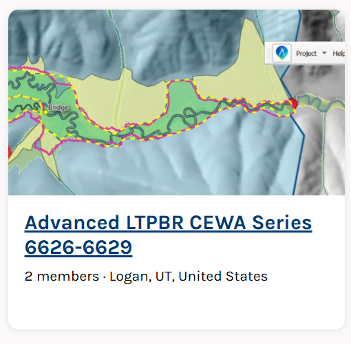
Community Page on Riverscapes Consortium for Advanced LTPBR CEWA Series 6626-6629

Event Page for 2025 Course

Event Page with Meeting Joining Details

Prerequisites and Preparing for Class

Background or Catch-Up Reading

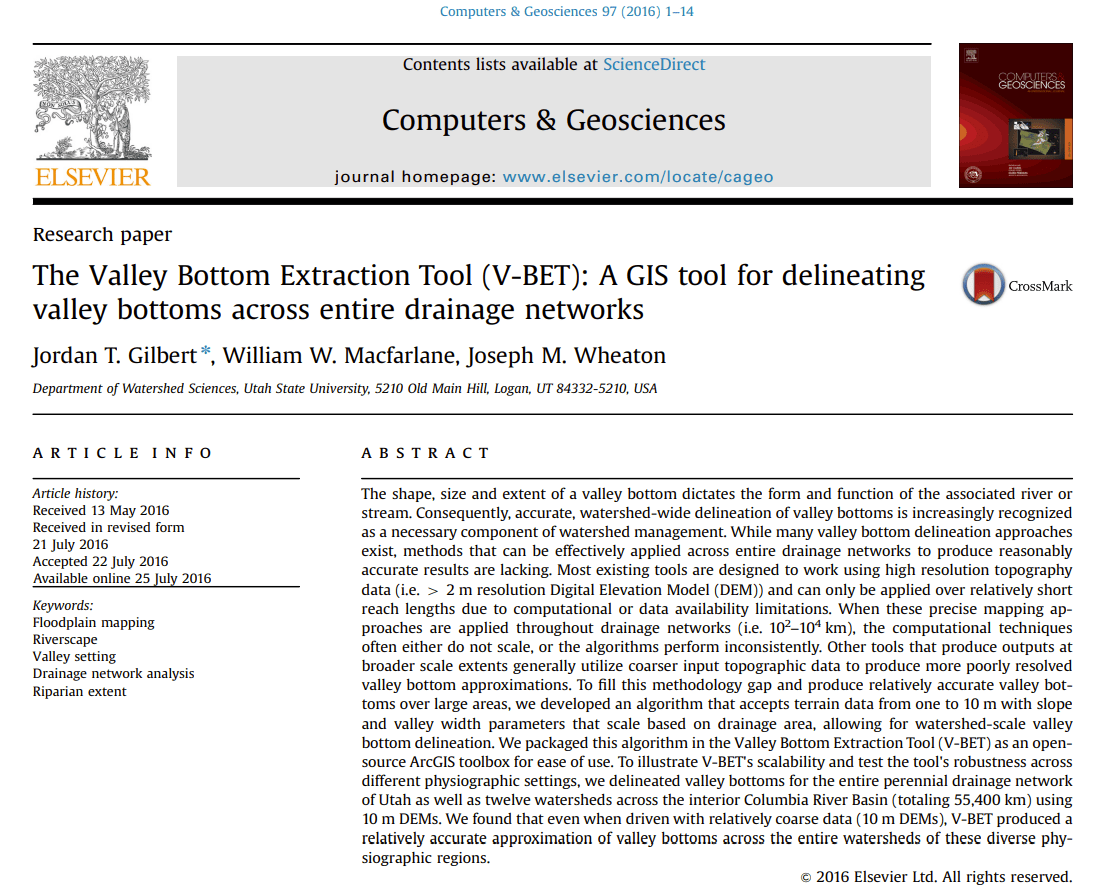
VBET

The original paper documenting the first version of the Valley Bottom Extraction Tool. It has undergone siginificant development since this paper, some of which will be covered in class.

Beaver Restoration Assessment Tool (BRAT)

The paper documenting the Beaver Restoration Assessment Tool (BRAT). This also documents some components of the Anthropogenic Context and Hydrologic Context Tools, which were split out of BRAT.

Confinement

Paper that documents the confinement algorithm and shows its application.

RCAT

The paper documenting the Riparian Condition Assessment Tool algorithm.

Software Requirements

Install QGiS and the QRiS and Riverscapes Viewer Plugins (see here).
Install SQLite Studio to perform SQL queries on model outputs in a non-geospatial environment.

warning

If you did not take the planning course, please review the software installation instructions and ensure you have QGiS, the QRiS plugin, and the Riverscapes Viewer plugin installed and working before the first day of class. If you need help with this, please show up on Monday morning at 8:45 AM instead of 9:00 AM.

Downloading and opening Riverscapes Projects

Because this course will involve retrieving data from the data exchange and opening it in the Riverscapes Viewer in QGIS participant should be familiar with the workflow below:

Go to the Riverscapes Data Exchange. If you haven't already, you will be prompted to create a login. You can create a new login, or link your account to your Google or Apple login. The home screen contains various cards to help navigate the Data Exchange. 'Explore, Search, Find' helps you find projects, organizations, and people. 'My Organizations' shows the Data Exchange organizations that you are a member of. 'My Bookmarked Items' shows items that you have bookmarked to return to later. 'Project Types' shows the main model types housed in the exchange with links to browse those specific model types.
Click on the 'Expore our Project Map' button in the 'Explore, Search, Find' card. This will open a web map that can be used to navigate to find projects.
At the top, there is a dropdown menu that allows you to filter by project type. Choose a project type you are interested in (from the Riverscapes Network Models types) and set the filter.
Either manually zoom to an area you are interested in, or use the embedded search ('Find a place') in the map and type in a place (e.g., a city name). Once you are zoomed in to a certain level, you will see polygon outlines of project boundaries.
Click inside of a project extent - this will pin a card showing the available projects of the selected type, for that extent. (If you hover over the small project extent polygon there are two buttons: one to zoom to the extent of the polygon, and one to filter your selection to projects with that extent.) Click on a specific project to go to the project page. A new page will open with the project name as the header. There are several tabs on the page, with the 'overview' tab selected by default. Click through the other tabs to explore the information the page contains.
On the top right (to the right of the project name) are several buttons: the 'bookmark' button, which allows you to bookmark the project to come back to later from your home landing page, the 'download' button to download the project to your local machine, the 'share' button share the link to the project, the 'open map viewer' button, which opens the project in the Data Exchange's integrated web GIS, and the 'copy project to clipboard' button. Click on the 'open map viewer' (globe button) to open the project in the web GIS.
In the web GIS, there is a project tree on the left side, which shows the structure of the project and the data layers in the project. The right side has a layers table of contents. Layers are added by double clicking them in the project tree, or right clicking them and choosing 'Add to Map'. Layers are removed by clicking the 'X' beside them in the table of contents. At the top of the layers panel is a 'Curated Views' dropdown. Curated views are combinations of coherent layers that are added to the map together. Bring layers into the map (and remove them) using both the project tree as well as the curated views to explore the layers that are contained in the project. Note that there is an 'identify features' button on the bottom left of the map. This button allows you to view the attributes of any feature of a feature class that you have open in the map.

info

While we actively maintain the curation of these projects (project structure and layer symbology), occasionally changes/updates cause issues. If a layer is not showing up when you pull it into the map the symbology likely needs updated. If you wish to file an issue for the team to respond to, you can do so in GitHub (requires a GitHub account), or our Help Desk(does not require an account).

The top left part of the screen has a project card. On the bottom right of the card is another 'download' button. Click the button to download a zip file of the project to your local machine (in the directory you created to easily access data for this course), and extract the zipped folder.
Open QGIS. You should have the Riverscapes Viewer plugin installed. If you do not see the instructions here. Click on the 'Riverscapes Viewer' button, then choose 'Open Riverscapes Project'. Navigate to the project folder that you downloaded. Inside the folder is a file called 'project.rs.xml'. This is the file that you select to open the project in QGIS.

tip

For more info on the functionality of the Viewer, see the documenation

Similar to the web viewer, a panel opens with a project tree, from which layers can be added to the map. Like the web viewer, projects can simply be viewed using the 'prebaked' symbology in the viewer. However, now you are operating in a fully functional GIS environment, and can acually perform spatial analysis on the data within the projects.

tip

For an overview of the Data Exchange and its functionality, see the videos on the documentation page.

Main Assignment

The main outcome of this workshop is to come up with a prioritized list of potential restoration sites within a geography with a minimum size, with appropriate conextual justification for the decisions.

Resources

Class Recordings

Details

Our morning sessions are recorded for your reference.

Monday

info

Forthcoming - Will post after class.

Tuesday

info

Forthcoming - Will post after class.

Wednesday

info

Forthcoming - Will post after class.

Thursday

info

Forthcoming - Will post after class.

Community Resources

These communities from the Riverscapes Consortium are great places to ask questions, connect with colleagues and share your work.

Advanced CEWA LTPBR Series Community

The community for connecting with others in this class and the advanced series of Adavanced LTPBR courses.

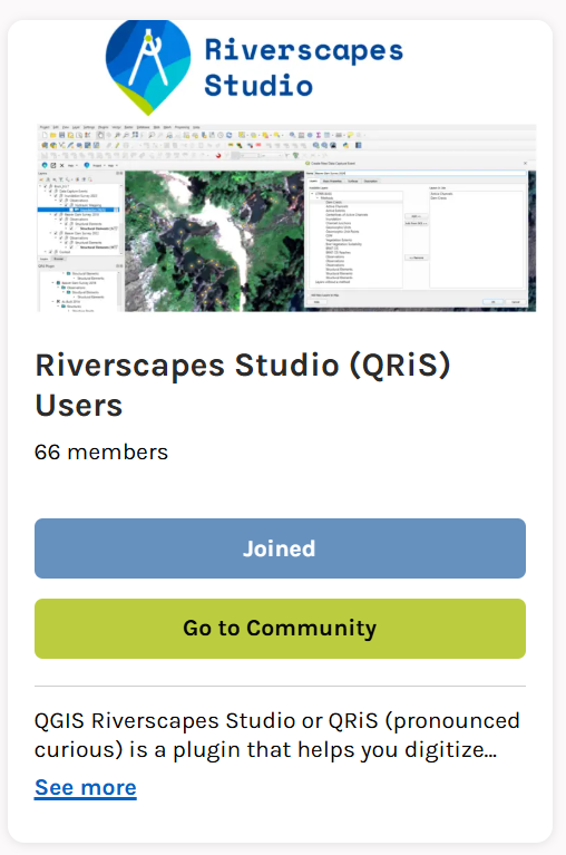
Riverscapes Studio Users

Community of QRiS Users. Stay up to date on latest releases, webinars, trainings, ask questions and share your work.

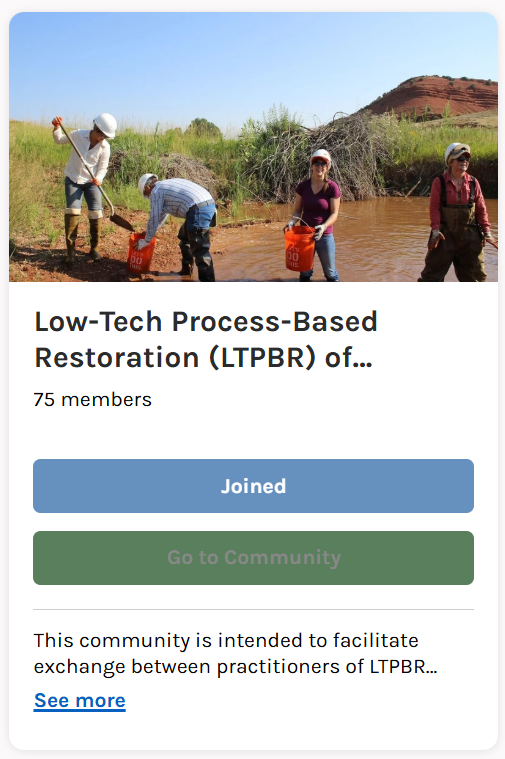
LTPBR of Riverscapes - Practitioner Community

This community is intended to facilitate exchange between practitioners of LTPBR anywhere in the world.

Assignment Resources

In Class Exercises

Data for Exercises

tip

You are welcome to download these projects as we use them in class, or download them all ahead of time. We suggest downloading them somewhere easy to navigate to (and making a favorite shortcut to that folder in QGIS) such as c:/0_RS/CEWA6629/.

Riverscapes Data Exchange Projects for Exercises

Metric Engine for Ogden River

Riverscape Metric Engine project for the Ogden River HUC10 watershed in northern Utah.

Rivercapes IGOs for Bear River

Riverscapes IGOs project for the Bear River watershed. This project type is a 'merged' RME where the DGO attributes from RME are attributed to the IGO points.

1. Overview of Screening & Prioritization

Using large-scale GIS datasets and geospatial models to plan and prioritize is particularly useful in the case where you have a large geographic extent across which you could work, and a limited budget for restoration. In such cases, you need to narrow down your extent to specific locations where it makes sense to work, and then prioritize them (e.g., based on potential for uplift) such that the dollars spent are being most effectively used.

If you have a small spatial extent (i.e., there is a predetermined, specific place to work in) screening and prioritization may not be necessary. Similarly, if you have enough budget to treat all of the riverscape under your purview, prioritization may not be necessary. Realistically, budget constraint generally require some level of decision making about where to work and what actions to perform.

A good workflow often involves utilizing available remote sensing/GIS data and model outputs as a first step to get an understanding of the systems you could work in, and start to screen and filter down to potential restoration sites. After this first step, visiting as many of the potential sites in the field is valuable to integrate information that you can't get at
remotely. Often times, seeing and thinking about riverscapes in person also helps to assess what additional information (beyond what you had gathered in your initial assessment) may be useful for decision making.

Slides

2. Riverscapes Metric Engine

a. RME Overview

RME has a lot of attributes in the output feature class. Descriptions of each field can be found here.

b. Inventory of Opportunities

Exercise: Across the Ogden River HUC10 watershed, determine the area of perennial riverscape (km²) that falls into each ownership category present (e.g., Private, State, USFS, etc.)

Open the RME project in QGIS using the Viewer plugin.
Bring in the Dominant Land Ownership (DGO) layer (Outputs > DGO Descriptive Metrics > Dominant Land Ownership (DGO)).
Right click on the layer in the table of contents and open its attribute table.
Click the "Select features using an expression" button on the top bar of the attribute table.
Select features for a given land ownership type by typing the expression "FCode" in (46006, 55800) and "ownership" = 'PVT' (to select private land ownership for example). To see all available ownership options, you can find the 'fields and values' option in the middle panel of the expression builder, expand it, then click on the 'ownership' field and the click 'All Unique' to see all available options. After executing the expression, the selected features should be highlighted.
Use the 'Basic statistics for fields' QGIS tool to sum up the area of the selected features. Make sure the correct layer is selected, and the 'Selected features only' box is checked. For the field, choose segment_area, which is the area in m² of each polygon. After running the tool, one of the statistics calculated is the SUM which can be converted to km² and noted down.
Repeat the process for the remaining land ownership categories.

Now lets do the same thing but using SQL queries instead of GIS operations.

Open SQLite Studio, and click on the 'Add a database' button on the top left.
When navigating to a file, make sure that the extension option (Save as type) is changed to 'all file types' on the bottom of th window (rather than just .db type files) and then navigate to the rme output geopackage (riverscapes_metrics.gpkg) and select it.
This will add the geopackage to the 'Databases' panel on the left. Once it is there click on it to highlight it, then press the 'Connect to the database' button to connect to the geopackage as a database (this should expand the database so you can see all of the tables inside).
Push the 'Open SQL editor' button on the top, and in the editor panel type the command: SELECT ownership AS owner, SUM(segment_area)/1000000 AS km2 FROM vw_dgo_metrics WHERE FCode IN (46006, 55800) GROUP BY owner ORDER BY km2 DESC then execute the command (blue play button). This one SQL command will provide all of the information you manually retrieved in QGIS.
Try another command where we get the same information but by stream instead of owner: SELECT stream_name AS stream, SUM(segment_area)/1000000 AS km2 FROM vw_dgo_metrics WHERE FCode IN (46006, 55800) GROUP BY stream ORDER BY km2 DESC. (Imagine how long it would have taken to manually do each individual stream using the QGIS method.) You could also create a table that shows each stream name and its area in each land ownership class by changing the query to SELECT stream_name AS stream, ownership AS owner, SUM(segment_area)*0.000247105 AS acres FROM vw_dgo_metrics WHERE FCode IN (46006, 55800) GROUP BY stream, owner. Note that in this example area is converted directly to acres in the query.

Often times, this type of tabular analysis is a useful first step for identifying areas where further spatial analysis can then be performed. Leveraging the capabilities of SQL by performing queries on the geopackage layers is an extremely useful and efficient way to perfrom this type of analysis.

c. Statistical analysis of metrics

Exercise: For a given stream in the HUC10 watershed (e.g., Middle Fork Ogden River), visualize the distribution of values for a continuous metric (e.g., valley bottom width (integrated_width)) using a histogram.

Open the Ogden River RME project in QGIS using the Viewer plugin.
Choose a metric with a continuous value (e.g., valley bottom width (integrated_width)) and bring it into the map (Outputs > Geomorphic Metrics > IGO Geomorphic Metrics > Integrated Width (IGO)).
Filter the output to a specific stream (e.g., Middle Fork Ogden River). Right click on the layer in the table of contents, choose 'Filter...', then type the expression "stream_name" = 'Middle Fork Ogden River' and pressing OK (NOTE: you could also copy the level path value for a given stream and use "level_path" = '<some level path value>' to filter).
Note how, because of the binning of values, the variation in the metric may not be well captured at the scale of a single stream. In this case, we will use a histogram to visualize the distribution of values for the entire stream, which will provide more context than the bins in the symbology. Find the 'Vector layer histogram' tool in the Processing Toolbox (you can search for it in the search bar at the top of the toolbox). Set the input layer to be the filtered, set the 'Attribute' to be integrated_width, increase the number of bins to 15, and press 'Run'. This will generate a histogram of all of the values for that stream.

3. Riverscape Network Models

a. The Model Waterfall

To help screen and prioritize, models provide three different types of information: 1) descriptive information that is useful for high level screening/filtering (e.g., land ownership, flow type, etc. as in the earlier exercises), 2) intentory information as in the earlier exercises where we quantified the area of riverscape or length of channel wihtin a watershed that meet a certain criteria, like we used above, and 3) some information to get at condition to help assess where needs restoration and where there is the greatest potential for uplift.

VBET Webinar

b. RSCLI

When you need to download more than a couple of projects from the Data Exchange, clicking on the download link, waiting for the file to zip, extracting it and saving it locally becomes time consuming and tedious. A command line tool exists to make this process faster and simpler. Documentation, including instructions on downloading the tool are found here.

c. Some exercize(s) using specific model types

Information from the network models is resolved at the reach scale (channel reach or riverscape reach; ~100s of meters), but it's time consuming and potentially impractical to look at values for every reach across a watershed. For this reason, it's often useful to roll-up or summarize the information at larger spatial scales. This allows for simple comparision between, e.g., sub-watersheds or individual streams. Comparisons that this scale can then inform what streams you zoom in on to assess the information at the reach scale, helping your efforts to stay targeted and efficient. These exercises use simple examples of summarization of outputs at the watershed scale and individual stream scale to assess potential for beaver-based restoration.

Demo (BRAT): Assessing restoration and conservation opportunities in one stream, contextualized by the rest of the basin.

Exercise (VBET): Compare the average low-lying proportion of valley bottom across two different streams.

This exercise demonstrates how a metric calculated by VBET (proportion of the floodplain that is low-lying) can be summarized along a given stream and the value compared to another stream.

Demo (RCAT): Investigating RCAT outputs and intermediates along a stream to assess opportunity

The exercises we've done so far have been fairly straightforward if the area you are assessing happens to be a HUC10 watershed and you can simply download the individual projects needed for analysis. But what do you do when your extent is larger, e.g., spanning multiple HUC10s, or very large, like an entire state. Downloading each project you need individually and manually merging features classes obviously would not be practical. We have had a few different strategies for dealing with this, most recently an interactive webpage for requesting data that we'll use here.

info

In these projects that are merged for large areas, we pull the metric/attribute values from the DGO polygons, but attach them to the IGO points. Points are much smaller (bytes) than polygons because they contain only a single vertex, so this strategy keeps the projects from getting too large (which both takes up hard drive space and causes GIS to crash). We use the DGO metrics to avoid complications that could arise from calculating statistics based on moving window metrics (e.g., overcounting area by adding up windows).

Exercise (Riverscapes IGOs): Using Riverscapes IGOs to filter down to a subset of streams across a large area

In this exercise, we will open a Riverscapes IGOs project together and come up with screening criteria to filter down our results to something more manageable.

d. Create a merged project for custom extent

The primary assignment for this course will be to use the techniques learned here to select some specific reaches within a large area where it makes sense to plan restoration/conservation actions. To do so, you will need a Riverscapes IGOs project for your area of interest (~HUC8 extent or larger).

Exercise: Generate a GeoJSON feature class of the extent that you want to create a project for.

In QGIS, click on the 'New Temporary Scratch Layer' to create a new feature class.
Name the layer and select 'Polygon' as the geometry type. Make sure the projection is set to EPSG:4326 WGS 84 (the default projection for riverscapes network models), and click 'OK'. The new layer will be added to your table of contents with editing already toggled on.
Click on the 'Add Polygon Feature' button in the digitizing toolbar and begin drawing the polygon extent you want. Single clicks add new vertices and a right click finalizes the digitization.
Click on 'Save Layer Edits' then toggle editing off. (If you decide you want to edit the polygon in any way, you can toggle editing on and use any of the editing tools to modify the polygon.)
Right click on the layer in the layers panel, navigate to 'Export' then click 'Save Features As...'. Change the format to GeoJSON, choose a file name and location, and then click 'OK' to export it. It will be added to the map and saved to the location you chose.

Exercise: Generate a custom project

Go to https://reports.riverscapes.net.
Choose the 'IGO Scraper' option. After clicking, there is some general information that is worth reading through to understand the project that will be created.
Click on 'CREATE THIS REPORT'.
For the 'Select Area' option, choose 'UPLOAD', then click 'UPLOAD GEOPACKAGE OR GEOJSON FILE' and navigate to the GeoJSON layer you created.
Verify the extent looks correct and click 'SUBMIT'.
Give the project a name, and optionally a memo, then click 'START'. You will be returned to the 'MY REPORTS' tab of the page, which will show the project you have requested and its status (which will be 'queued' then 'running' at first).
When the project is finished generating, click on the blue folder icon on the right to download a zipped file of the project.

4. Reach Typing

Reach typing serves two primary purposes in the context of screening and prioritization: 1) It helps inform which metrics from the models may be relevant to condition in different settings, based on the natural regimes of those settings. 2) When you are working in a given reach type, it helps find 'control' or similar reaches with varying condition to contextualize the site and its restoration potential.

Exercise: Come up with some criteria for a specific reach type based on a reach you are interested in, and apply it to the Riverscapes IGOs project you created. Describe the reach type, and report on the riverscape area and length of that reach type across the project extent.

5. Bringing it all together

To complete the assignment, use the Riverscapes IGOs project you created to select some areas for potential restoration/conservation work. This involves the three 'steps' we've discussed in the class:

Apply any relevant filtering criteria to the IGOs to narrow down the project to places you could potentially work (e.g., by ownership, state, flow type (FCode)) etc.
After applying the filtering criteria, calculate some inventory statistics to compare opportunities (e.g., what is the riverscape area, of some/all of the unique streams remaining after filtering? What is the riverscape length split up by ecoregion of the riverscapes that meet your criteria?)
Using this inventory information further narrow down your selection. To a few streams/reaches/subwatersheds. Based on the reach types of your selection, choose some of the metrics that are relevant to condition and summarize them at the riverscape/level path scale. Finally, look at the variability in these metrics at the reach scale to assess variability in condition and where opportunities may exist.

tip

Adding custom/regional datasets to analyses using DGOs as a sample frame While we didn't directly cover it in this class, simple spatial joins in GIS can allow you to add new attributes to the existing metrics to bring in any other additional information that may be relevant to your goals and objectives for restoration (e.g., species distribution layers).