In Workshop 1, we created the building blocks to start the project planning process.
After Workshop 1, you should have:
- Installed QRiS and the Profile Tool
- Downloaded our example project from the Data Exchange
- Brought contextual datasets into your project (DEM, NHD Flowlines, Land Ownership)
- Delineated Areas of Interest (AOIs)
- Imported imagery
With these building blocks established, we’re ready to begin the LTPBR project planning process.
Sample project data (raw) Sample project data (already processed, as we’ll do in this guide)
In Tutorial 2, we’ll add more context to our project, digitize the riverscape, map risk and recovery space, and create a planning container and sample frames. The planning process is what sets us up with understanding of current conditions and recovery space to produce realistic designs.
The Webinar
Intro Slides
Webinar Recording
Webinar Transcript
Autogenerated transcript of webinar (PDF).
Self-Paced - Tutorial 2
Desk Guide - Survey of Features
Download the Desk Guide for this workshop here
Valley Mapping
Our project already has [existing data] from the first workshop.
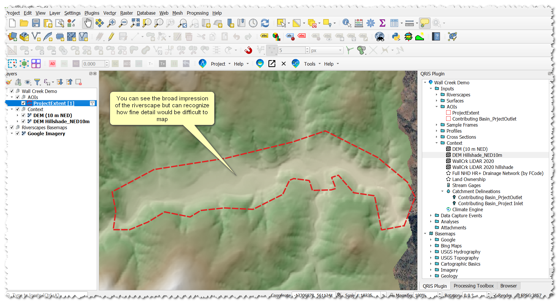
We have a DEM in our context folder. Add the DEM to the map by double-clicking the layer, or right-click -> add to map.
As you can see, at this scale, our 10m DEM shows a broad impression of the riverscape and can be used with free satellite imagery for a cursory mapping of our riverscape. However, if higher resolution surfaces are available (e.g. Lider or higher resolution imagery) they can make desktop mapping of your riverscape easier.
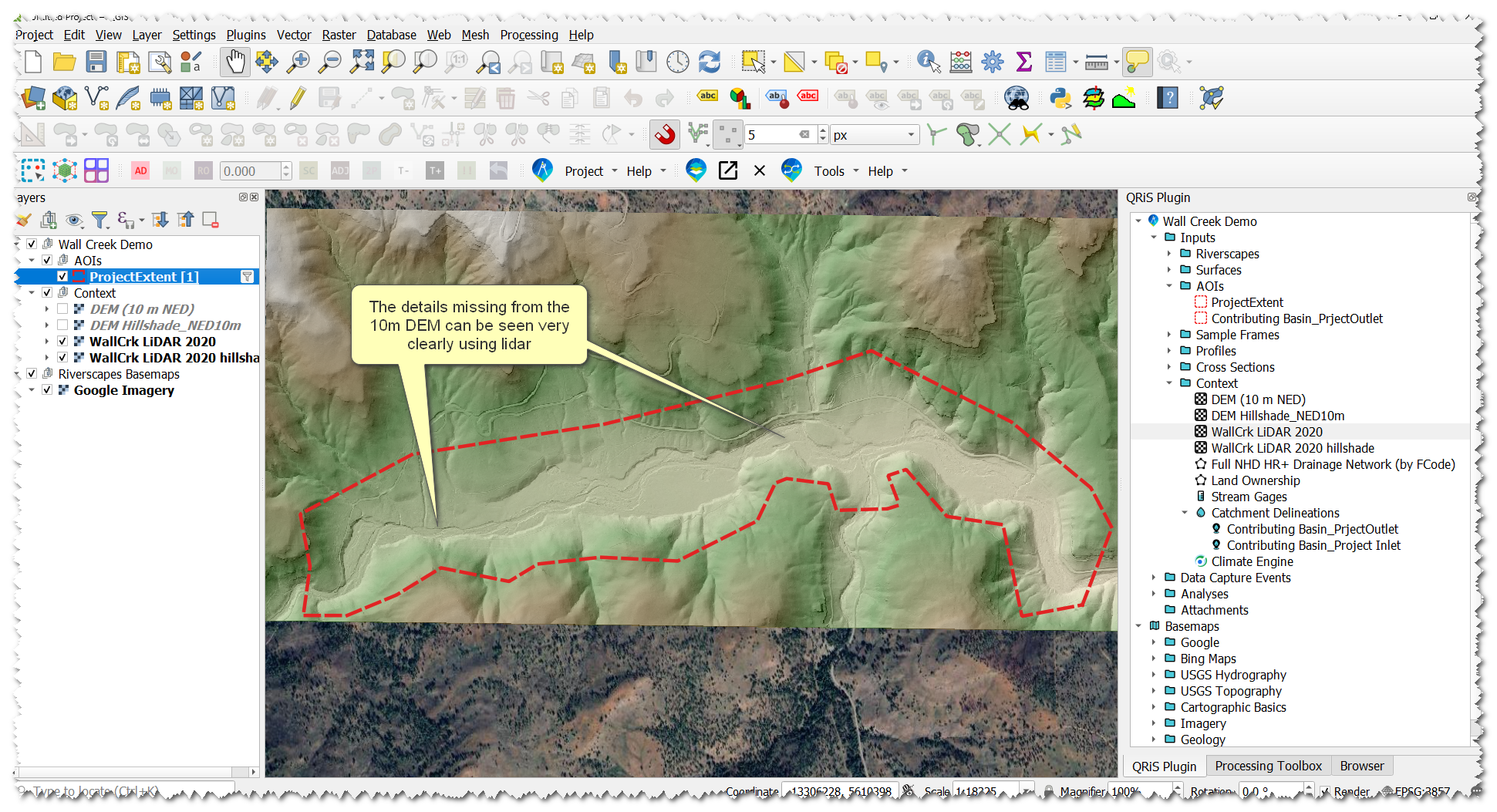
Add Contextual Basemaps/Imagery
Add DEM and Hillshade
- In your QRiS project -> right click the Context node -> Import Existing Context Raster
- Browse to your LiDAR dataset
- Set Raster Type to DEM.
- Leave the “Create Hillshade” box checked, so both the DEM and its derived hillshade load into the project
Demo Video
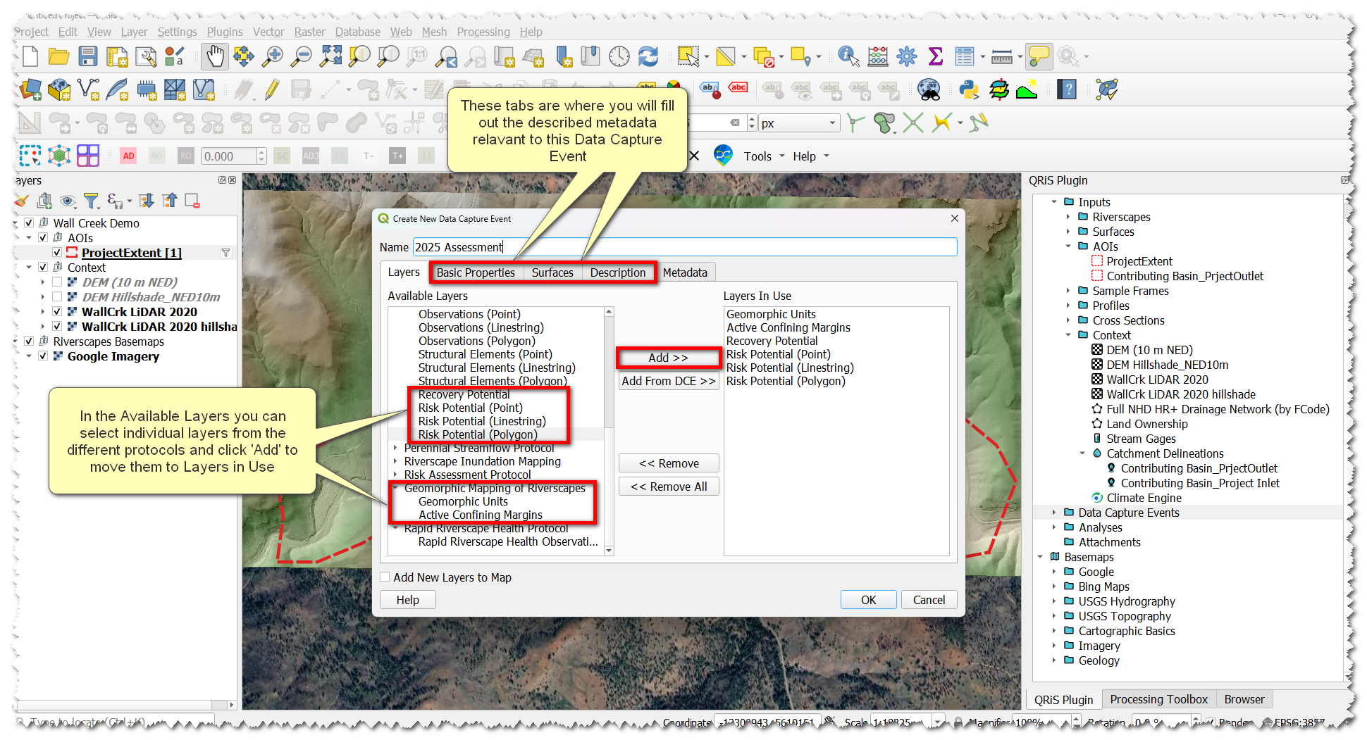
Create a Data Capture Event (DCE)
Using our high resolution imagery and our LiDAR hillshade, we will begin to map out our riverscape.
- Right-click Data Capture Events node -> Add New Data Capture Event
- Select Geomorphic Mapping of Riverscapes in the pop-up window. Click Add.
- Under LTPBR Protocol, add layers:
- Risk Potential (points, lines, polygons)
- Recovery Space
- Name the DCE something useful, like 2025 Assessment
- In the Basic Properties tab, set the data or date range based on LiDAR captured dates
- In our example, it was captured between 11/4/2019-8/19/2020
- Under Surfaces, select your LiDAR surface and high-res imagery
- In the Description tab, write a brief description of this DCE. A good description in this example would be, “This DCE represents the planning portion of this project. It is based on high resolution imagery and LiDAR.”
Demo Video
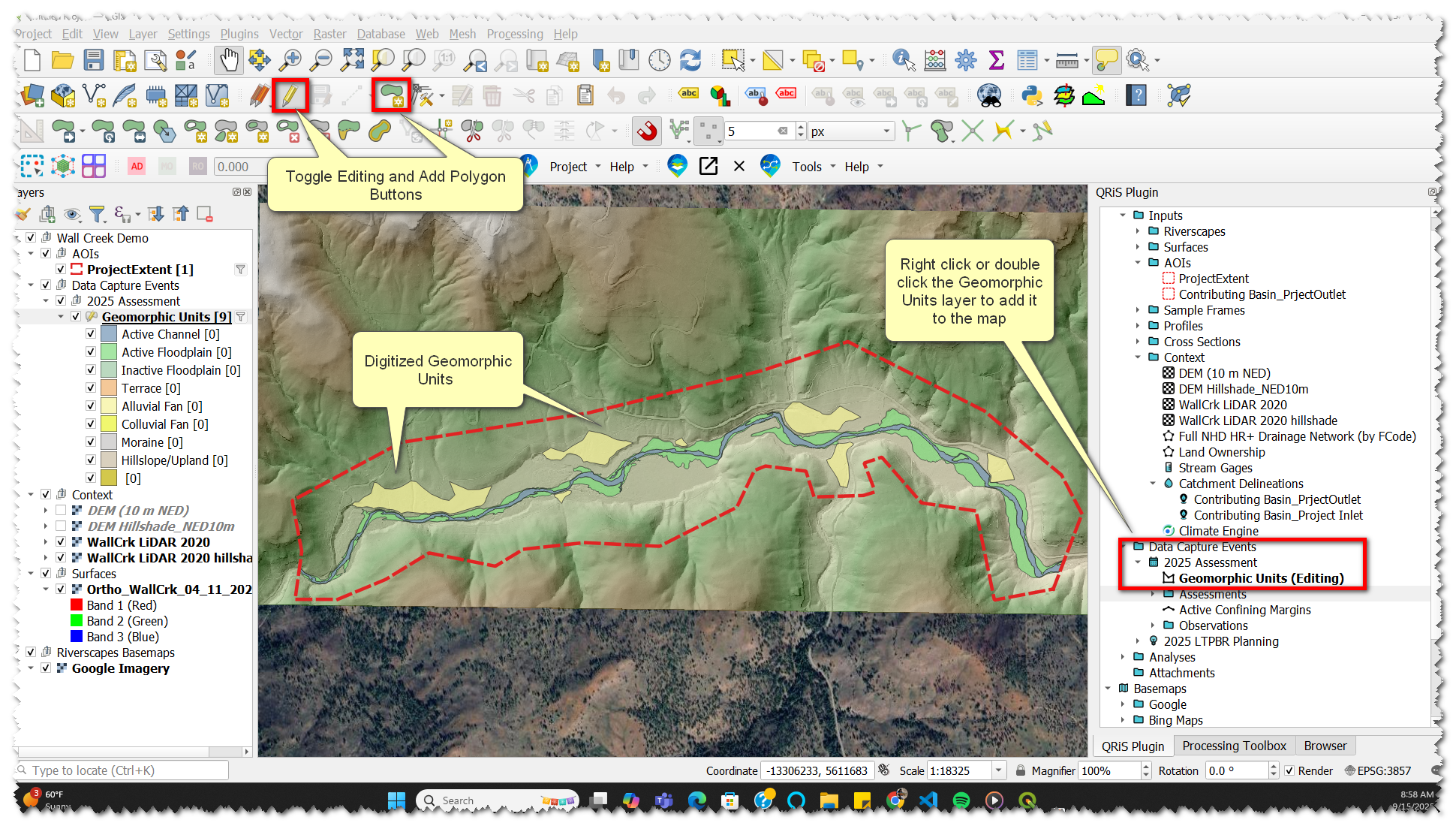
Map Geomorphic Units
- Add the Geomorphic Units layer to the map (either by double-clicking, or right-click -> add to map)
- With the Geomorphic Units layer selected, toggle editing.
- Click Add Polygon Feature. Using this tool, digitize terraces and fans, then digitize your active channel.
- Note: This is a great place to start using the Profile tool. The Profile Tool provides a better understanding of a landscape than visual identification, resulting in better mapping accuracy.
- Pull cross-sections from hillslope -> valley bottom -> hillslope to help verify valley bottom boundaries. Try it again across sections of the riverscape you suspect are hillslope transitioning to valley bottom to fan. This can help you draw your unit boundaries more accurately.
- Note: This is a great place to start using the Profile tool. The Profile Tool provides a better understanding of a landscape than visual identification, resulting in better mapping accuracy.
- Save edits by clicking the toggle editing button and save on the pop-up window
Demo Video
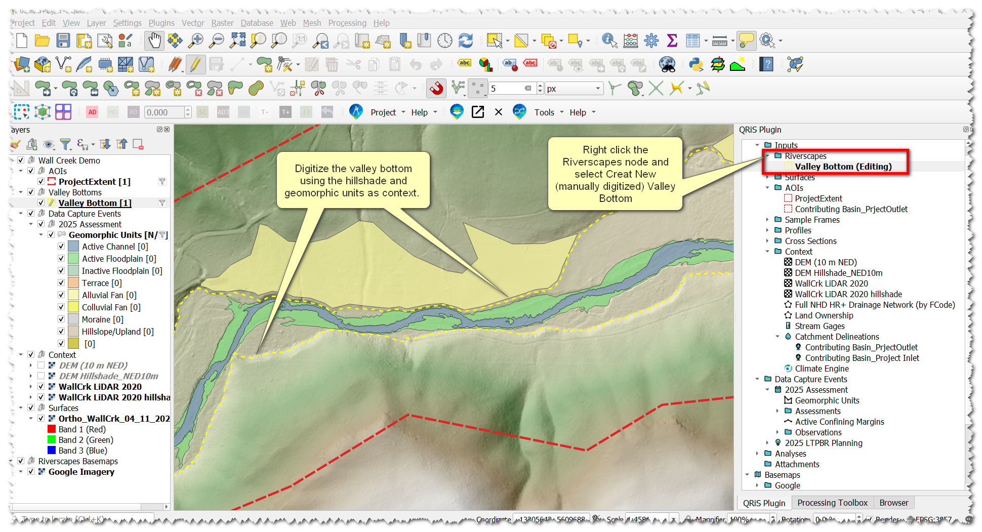
Map the Valley Bottom
- Right-click Riverscapes node -> Create New (Manually Digitized) Valley Bottom. Name and describe the layer in the pop-up window.
- With the new valley bottom layer selected -> toggle editing.
- Click Add Polygon Feature.
- Digitize valley bottom polygons, informed by the hillshade and valley geomorphic units we just digitized. The valley bottom only (this layer) includes active channel and floodplain, and excludes fans and terraces.
- Save edits by clicking the toggle editing button and save on the pop-up window.
Demo Video
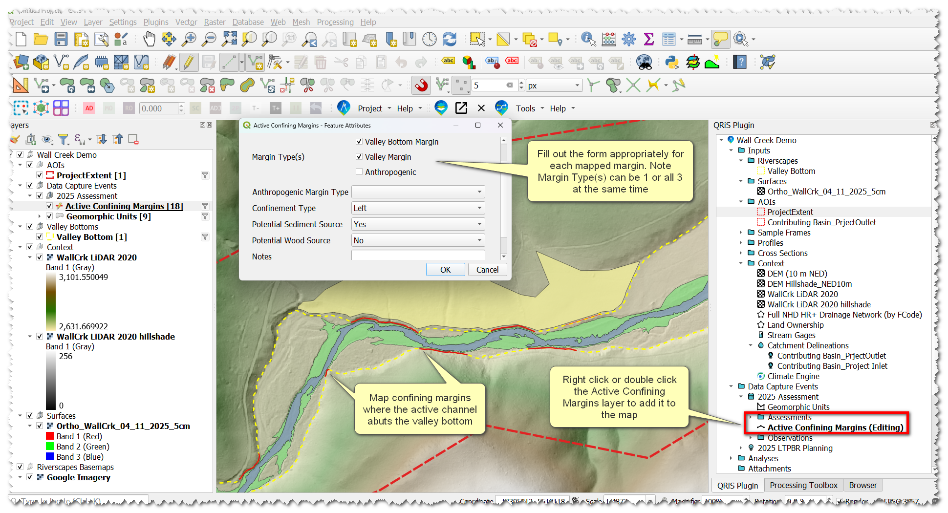
Map Active Confining Margins
- In your DCE -> Active Confining Margins layer -> double-click or right-click -> add to map
- With the Active Confining Margins layer selected, toggle editing.
- Digitize places where the channel abuts a confining margin. Select the appropriate attributes associated with each mapped margin
- Save edits by clicking the toggle editing button and save on the pop-up window.
Demo Video
Risk Mapping
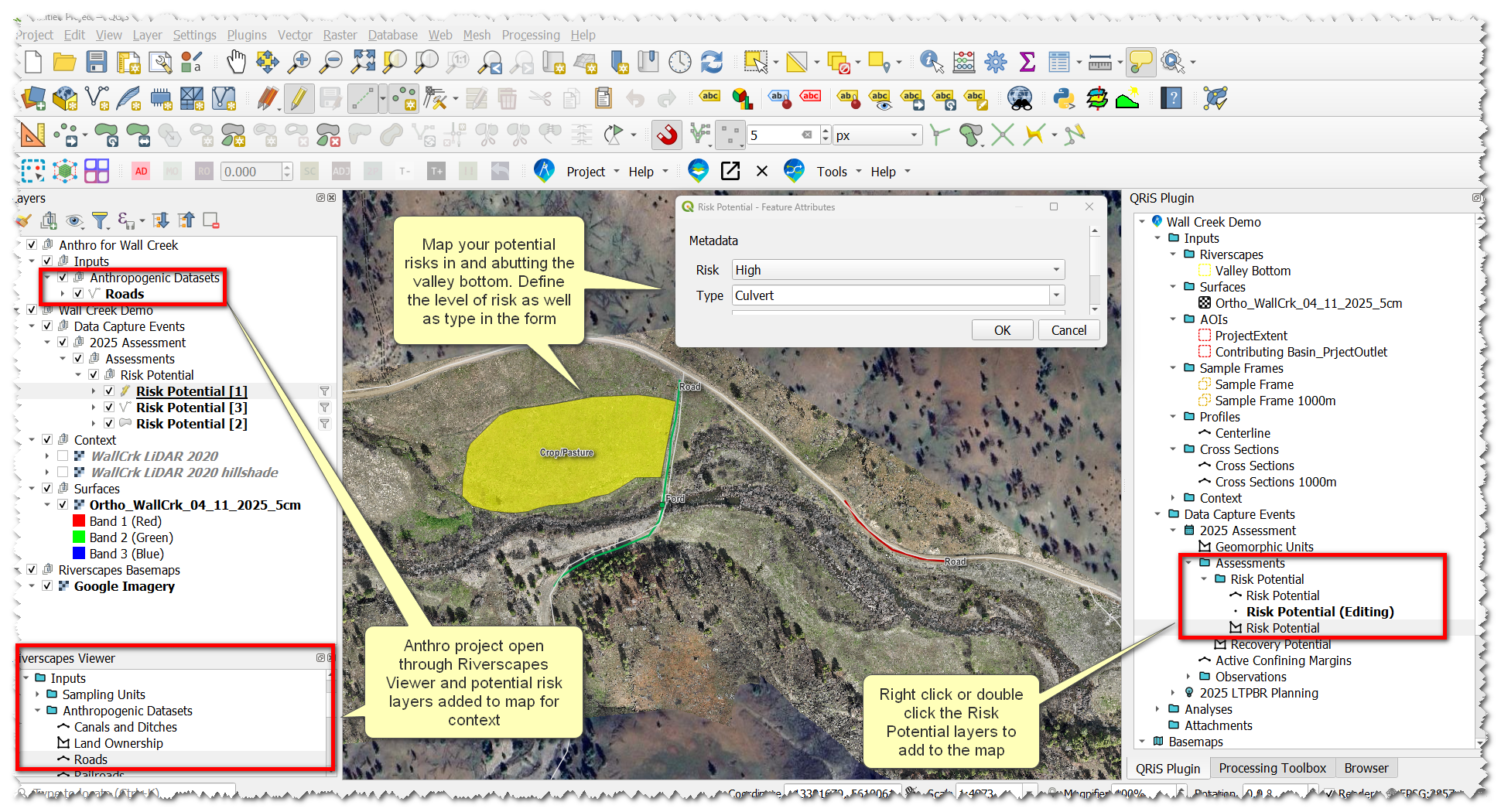
Download and load an Anthro Project to aid in risk mapping
- Right-click the project name in QRiS -> Browse Data Exchange Projects -> Download Anthro project
- Back in Riverscapes Viewer -> select Open Riverscapes Project -> navigate to the project.rs.xml file in your downloaded Anthro project
- In the Riverscapes Viewer panel, add potential risk layers to the map (layers such as roads, canals, land ownership, etc). We’ll use these as the basis for delineating your risk layers next.
- Add one of your QRIS risk layers to the map and toggle editing. There are three different Risk Potential layers: points, lines, and polygons. Digitize these as:
- Polygons: risk you may need to create a boundary on, like a building or pasture
- Lines: roads, canals, etc
- Points: culverts, bridges, etc
- Assign risk attributes for features including type and severity
- Repeat on each layer individually as necessary.
Demo Video
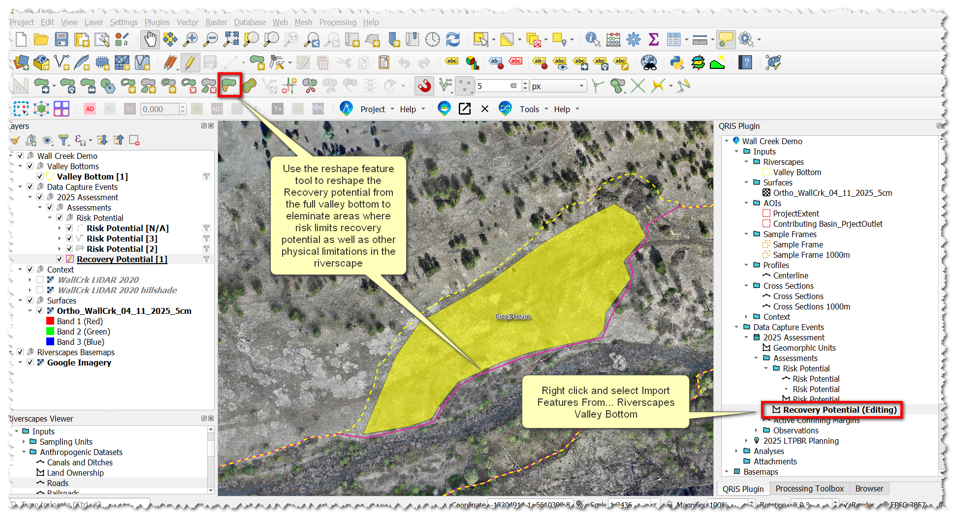
Recovery Space Mapping
The riverscape valley bottom is the baseline for recovery space, so we’ll start with that previously-digitized information. This step will duplicate the Valley Bottom geometry into the recovery space layer where we can make necessary edits without having to start from scratch.
- Right-click on the recovery space layer -> Import Features from Riverscapes Valley Bottom
- Toggle editing on the layer. Use the Reshape Features digitizing tool to make edits where necessary.
Here, we can look at the risk layers we digitized and determine what we can actually recover in the riverscape. Consider what portions of the active floodplain are recoverable, versus parts separated by a berm, levee, or other limiting factor not involved in risk mapping.
Map Additional Context Layers to Aid in Design
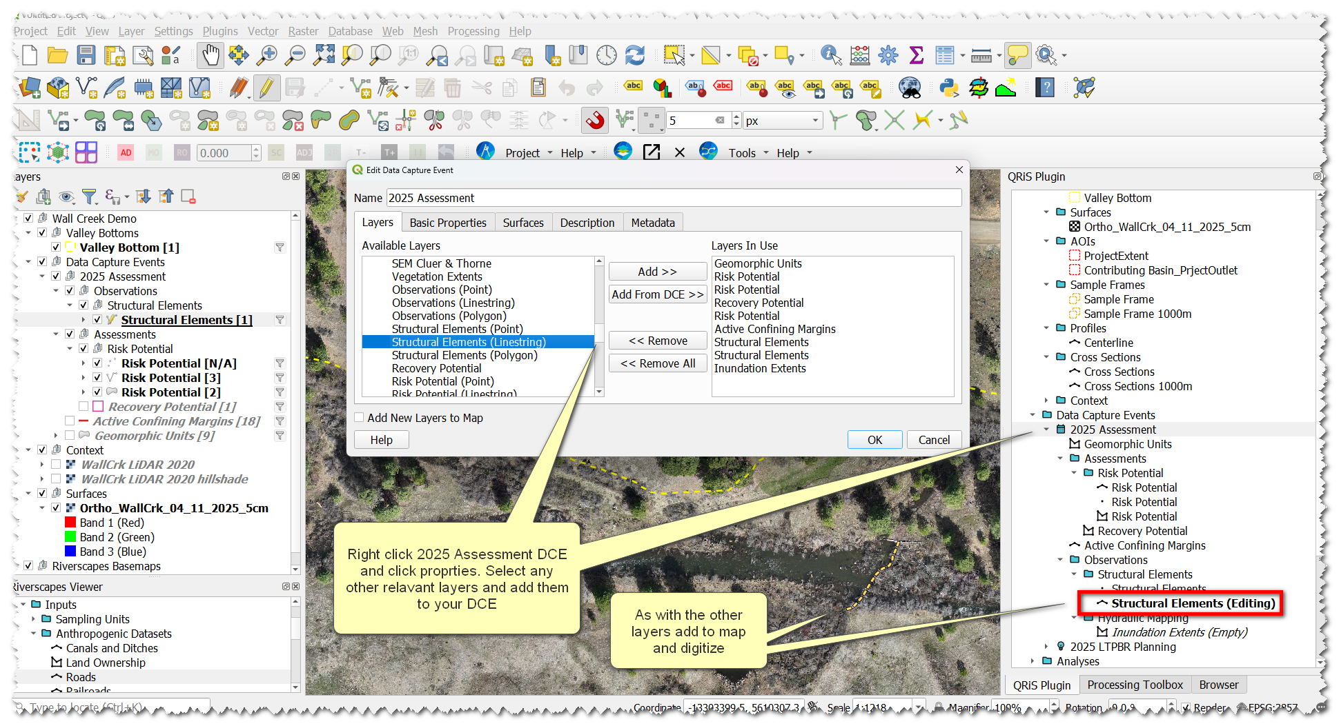
- Right-click your Data Capture Event -> Properties -> add additional layers to map (e.g. riparian vegetation, structural elements, inundation, etc)
- Digitize these layers as needed
Demo Video
Create a Planning Container
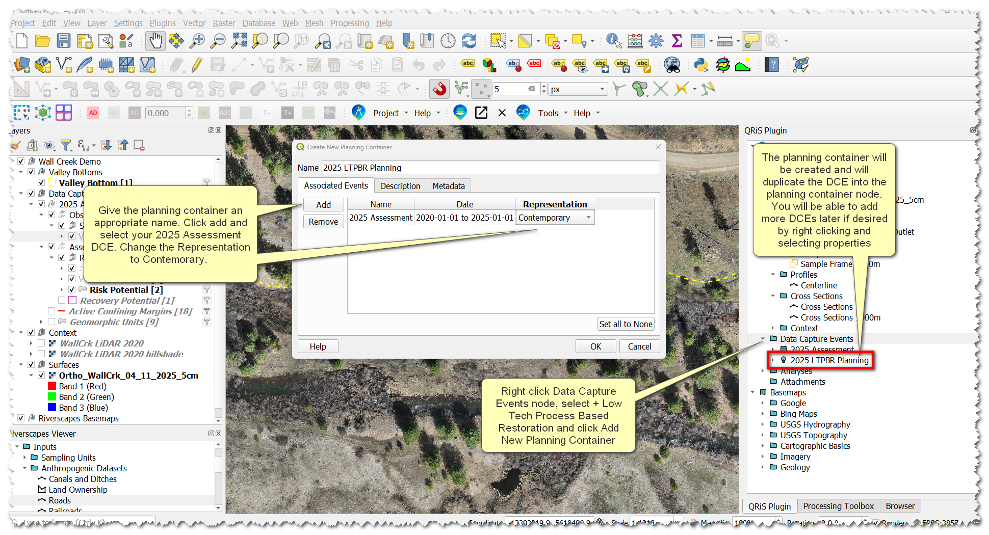
- Right-click Data Capture Events Folder -> +Low Tech Process Based Restoration -> Add New Planning Container
- In the pop-up, name it something useful, like 2025 LTPBR Planning. Click add -> select 2025 Assessment DCE. It will now populate the table. Change its representation to Contemporary.
Ideally, a planning container would also have both a Historic and Predicted DCE. A planning container simply copies DCEs into a new parent folder, which you’ll reference as the basis for LTPBR Design, when we get there.
Demo Video
Create Sample Frames
Sample Frames are what QRIS uses to calcualte metrics(i.e. zonal statistics) within as part of analyses. Sample Frames can be any polygon, but here we’ll consider two specific ways QRIS supports to create sample frames of riverscapes: i) using derived cross sections and ii) manually digitized cross sections (or reach breaks). If you want standardized reach lengths use derived cross sections. If you want to be in control of reach breaks then manually digitize cross sections. You may want to do this if there is a change in land ownership or a change in riverscape characteristics.
Sample Frames from Derived Cross Sections
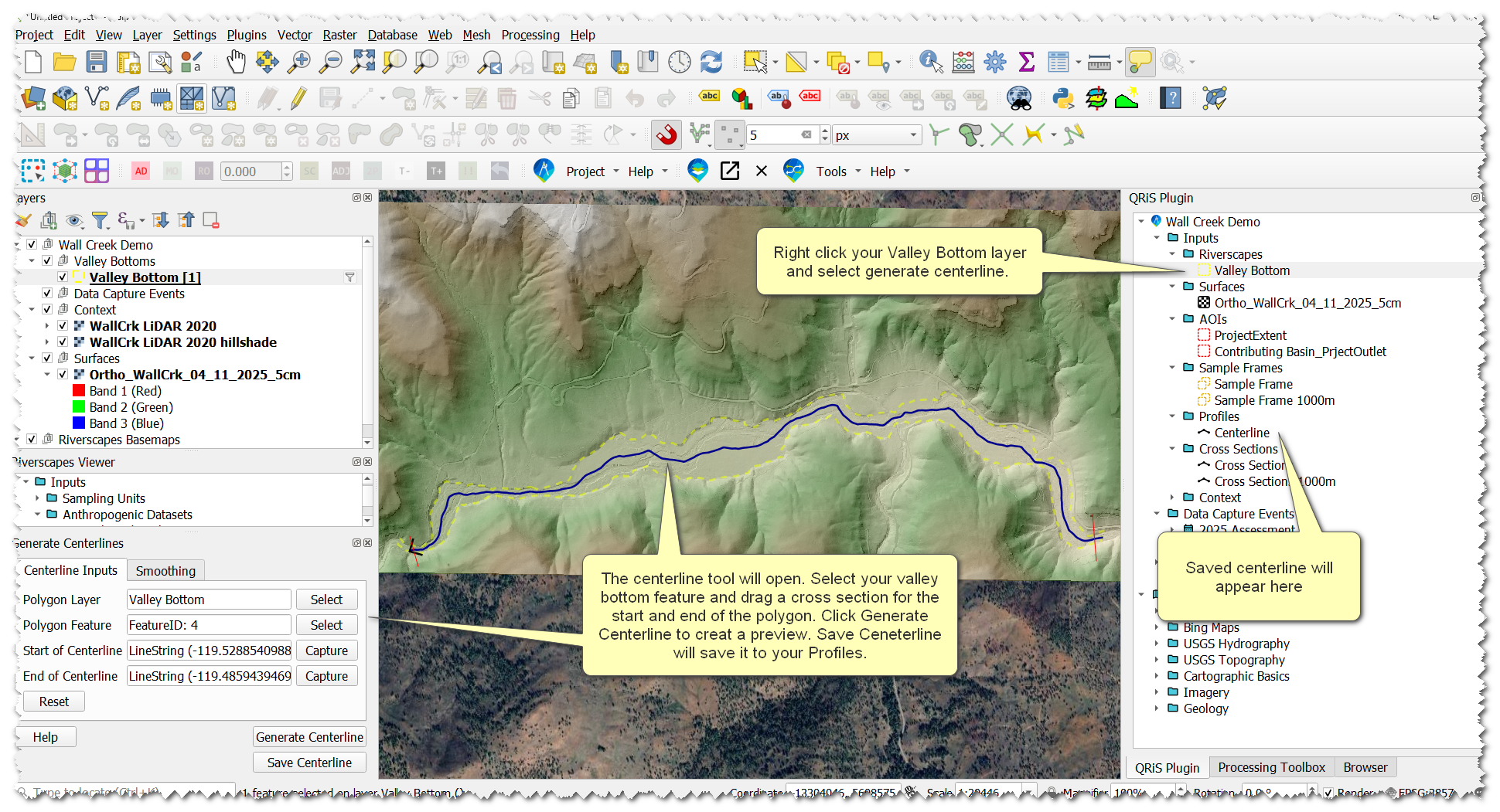
- Right-click the Valley Bottom layer -> Generate Centerline
- Use the centerline tool to create and save a centerline to your project
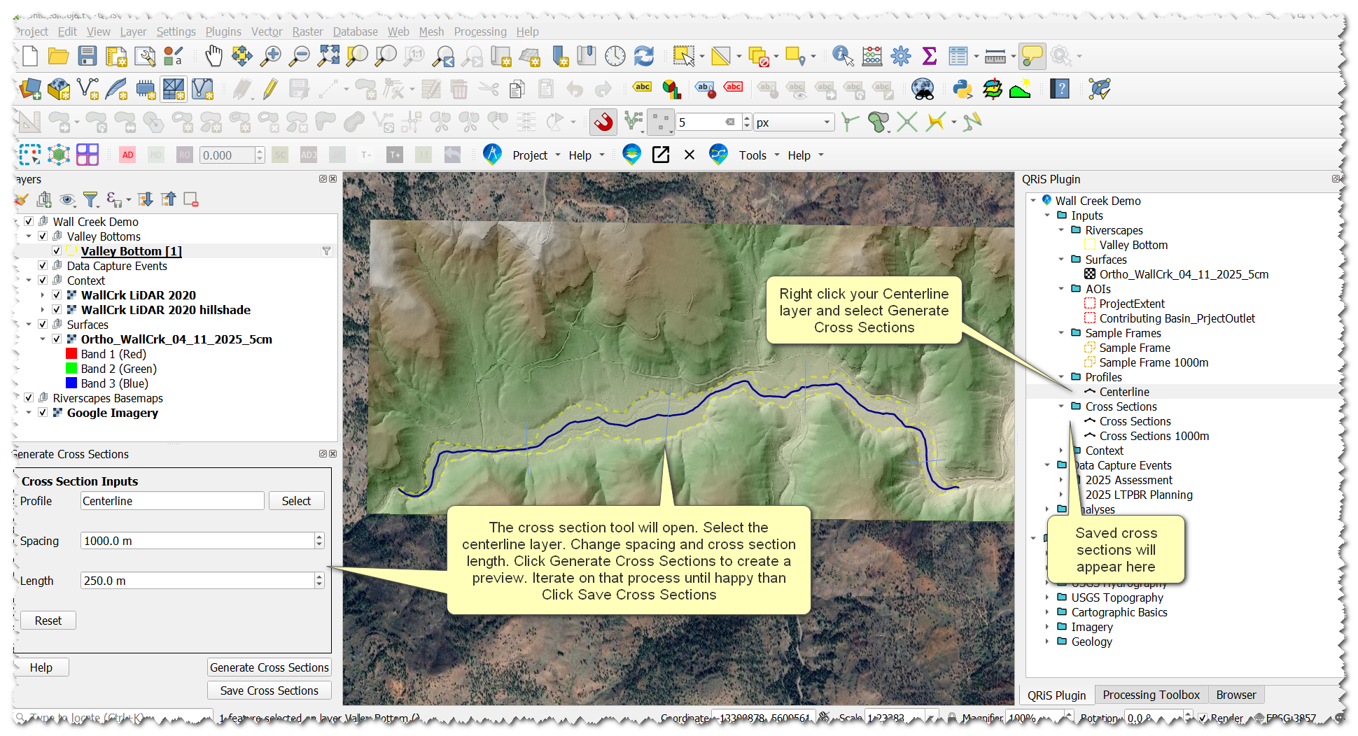
- Right-click the Centerline layer -> Generate Cross Sections
- Use the cross section tool to create and save cross sections to your project
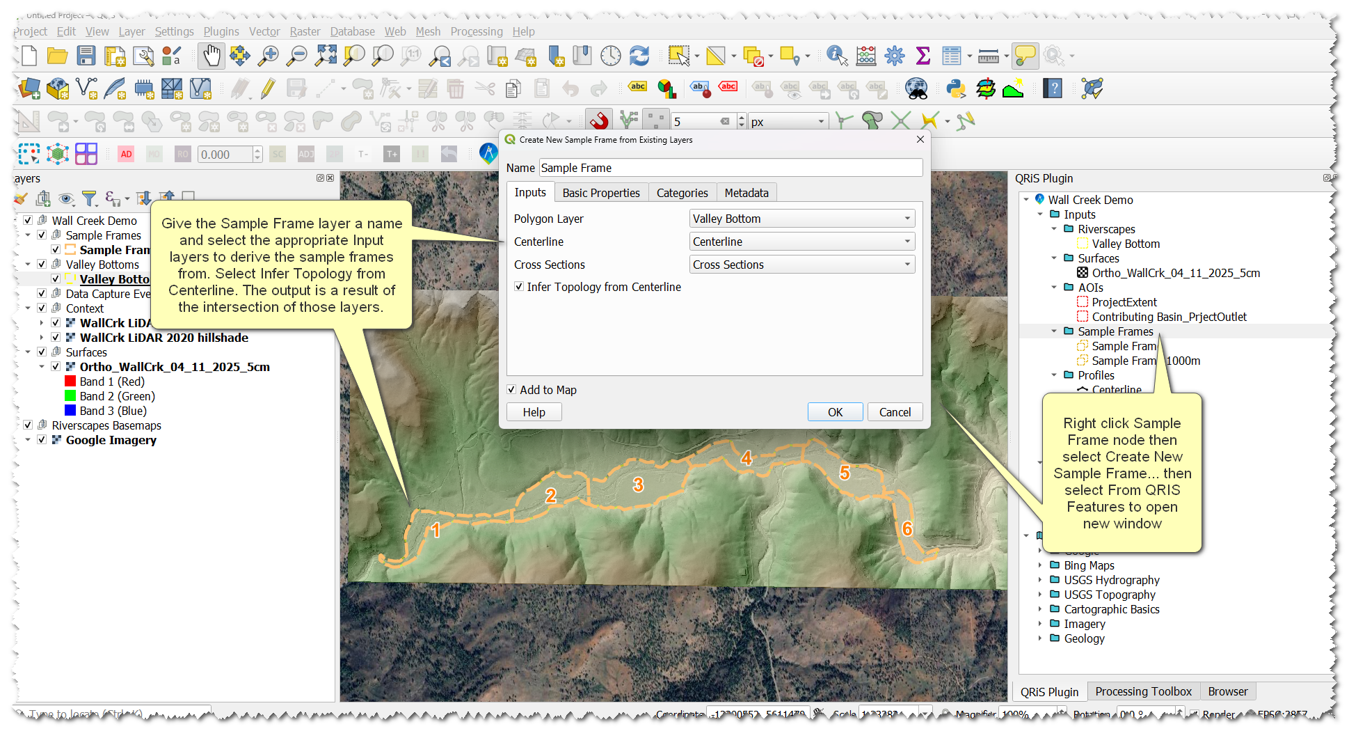
- Now, we have the building blocks to create a sample frame. Right-click the Sample Frames folder -> Create New Sample Frame -> From QRiS Features
- In the pop-up window, select the input layers to build a sample frame from(this will autopopulate with the layers you just created). Give it a helpful name. Check Infer Topology from Centerline.
Sample Frames from Manually Digitized Cross Sections
- Right-click the Cross Sections folder -> Create New (Manually Digitized) Cross Sections
- Add the layer to the map, then edit and digitize your cross sections. Ensure cross sections extend beyond either side of your valley bottom polygon.
- Once completed, right-click the Sample Frames folder -> Create New Sample Frame -> From QRiS Features.
- In the pop-up window, select the input layers to build a sample frame from. Give it a helpful name. Check Infer Topology from Centerline.
Demo Video
Create an Analysis and Calculate Metrics
Now that we have created sample frames we can use those to create an analysis and calculate metric values derived from features we digitized.
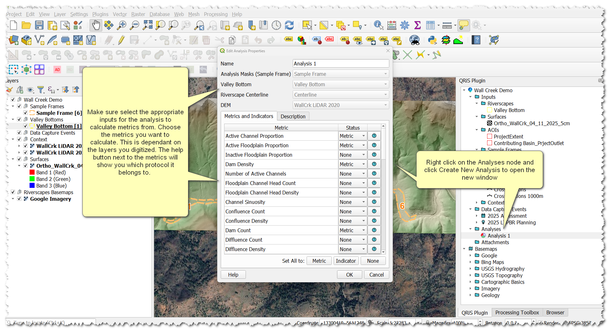
- Right-click the Analyses folder -> Create New Analysis
- Give the Analysis a name
- Select the sample frame layer you want to use to calculate metrics in
- Select the appropriate valley bottom layer, centerline layer, and DEM layer
- You will see a large list of metrics to select from. Click none at the bottom-right to set all metrics to none. Setting all to none allows you to go through and only choose the ones you want to calculate. Change the dropdown to metric on the following metrics:
- Dam count
- Dam density
- Jam Count
- Jam Density
- Active Floodplain Proportion
- Active Channel Proportion
- Proportion of Riverscape with recovery space
- Click OK
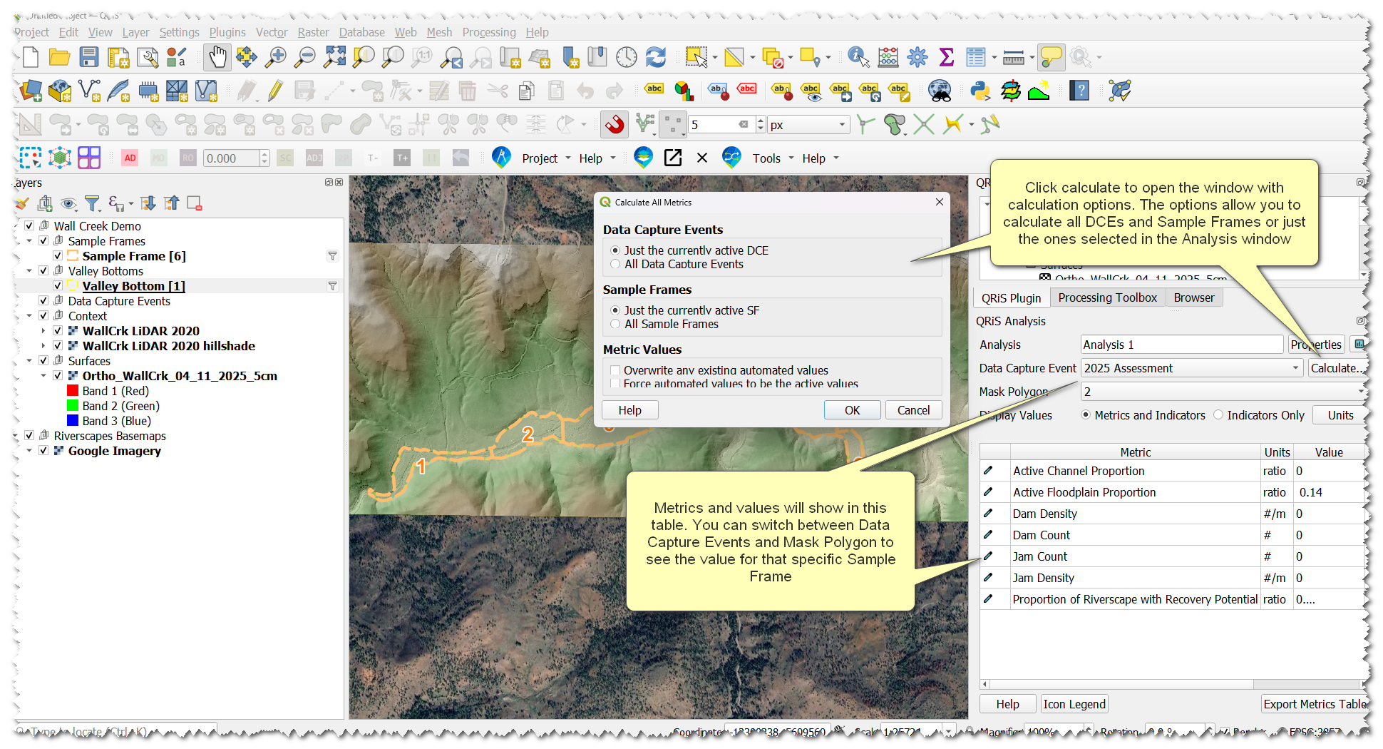
- On the window that pops up click calculate
- On the new window select All Sample Frames and click ok
- Values will calculate and populate in the table of metrics. Under the Mask Polygon Dropdown you can switch between your different sample frames to see the different metric values.
Metrics can be recalculated at any time and values can be overridden with manual values if necessary. More help can be found on the Analyses help page.
Demo Video